Scientific Peer Review, ca. 1945

いろいろな気候インデックスとの相関

*
*
NOAA　ESRLの
Linear Correlations in Atmospheric Seasonal/Monthly Averages
http://www.esrl.noaa.gov/psd/data/correlation/というページで各種気候インデックスといろいろな物理量の相関がプロットできる。


NINO3.4と表面温度の相関　(12月から2月）
日本は暖冬傾向だが、北日本でははっきりしない。
参考：気象庁

北極振動と表面温度の相関　(12月から2月）
日本は正の相関である。つまり北極振動が負だと寒冬の傾向がある。
参考：気象庁

北極振動 気圧場

*
*
2008年と2009年の気圧場（1000hpa Geopotential height）を比較する。
2009年は北極振動のパターンと逆の符号（負のフェーズ）の傾向が強い。

以下プログラム。

• python interface for grads
• matplotlib
• numpy
• basmap toolkit

を使用。
データはOpendapとい仕組みでNOAAからNCEP/NCARのデータを取得

from grads.ganum import GaNum  # for python interface for grads

from mpl_toolkits.basemap import Basemap  # for Basemap toolkit
import matplotlib.pyplot as plt
import numpy as np


for nyear in [2008,2009]:
# data import using python interface for grads
    ga = GaNum(Bin='grads')
    fh=ga.open("http://www.esrl.noaa.gov/psd/thredds/dodsC/Datasets/ncep.reanalysis.derived/pressure/hgt.mon.mean.nc") # data open
    ga("set time dec%(nyear)s" % locals())
    ga("set lat 0 90")
    ga("q file")
    ga("set lev 1000") # 1000 hpa
    hgt=ga.exp("hgt")
    del ga

    lat=hgt.grid.lat
    lon=hgt.grid.lon

# map
    fig=plt.figure()
    ax = fig.add_axes([0.1,0.1,0.8,0.8])
  
    map = Basemap(projection='nplaea',boundinglat=10,lon_0=135,resolution='i')
    map.drawcoastlines()
    map.drawmapboundary()
    lons,lats=np.meshgrid(lon[:],lat[:])
    x,y=map(lons,lats)
    map.fillcontinents()
    cz=map.contour(x,y,hgt[:,:],np.arange(-100,300,20))
    plt.clabel(cz,fmt="%3.0f")
    plt.title("Geopotential height (m): Dec %(nyear)s " % locals())
    plt.savefig("gpt_%(nyear)s.png" % locals())
    plt.show()

北極振動 Rで統計 グラフ編

* *

前回の続き

#boxplot
scripts="""
png(’boxplot.png’)
boxplot(rdatain)
dev.off()
"""
r(scripts)

去年の12月の値は「外れ値」にはなっていない

#hist
scripts="""
png('hist.png')
hist(rdatain,seq(-4, 4, 0.4),prob=TRUE)
x<-seq(-4, 4, 0.2)
lines(x, dnorm(x, mean=mean(rdatain), sd=sqrt(var(rdatain))), lty=3)
dev.off()
"""
a=r(scripts)

#cdf plot
scripts="""
png('cdf.png')
plot(ecdf(rdatain), do.points=FALSE, verticals=TRUE)
x<-seq(-4, 4, 0.01)
lines(x, pnorm(x, mean=mean(rdatain), sd=sqrt(var(rdatain))), lty=3)
dev.off()
"""
r(scripts)

#qqplot
scripts="""
png('qqplot.png')
qqnorm(rdatain)
qqline(rdatain)
dev.off()
"""
r(scripts)

正規分布より分布がせまい。

北極振動 Rで統計

北極振動　12月だけを抜き出しの続き

12月のデータだけ抜き出して、Rで統計処理する。 Rpy2を使う。
まずは以下のように準備。readAOとpickup_monthは以前作ったもの。

AO_rpy2.py 

from readAO import readAO # read AO data
from pick_month import pick_month # pick month
#
import scikits.timeseries as ts
#
import rpy2.robjects as robjects


# read AO data
AOindex_series=readAO()


# pickup December
AOindex_dec=pick_month(AOindex_series,month=12)


#remove missig value
data=AOindex_dec[AOindex_dec.mask==False].data


# for R
rdata=robjects.FloatVector(data)
robjects.globalEnv["rdatain"] = rdata
r=robjects.r

それで、

a=r('summary(rdatain)')

または

a=r.summary(rdata)

または

summary=r['summary']
a=summary(rdata)

いずれも同じ結果

print a
Min. 1st Qu. Median Mean 3rd Qu. Max.
-3.41300 -1.24200 -0.08762 -0.19740 0.82490 2.28200

print a[0]
-3.413

print a.names
[1] "Min." "1st Qu." "Median" "Mean" "3rd Qu." "Max."

b=a.r["Mean"]
print b
Mean
-0.1974

b[0]
-0.19739999999999999

print a.subset(1)
Min.
-3.413

参考
Rで統計: データ集合中の最大、最小、平均、中央値 - summary()関数http://www.yukun.info/blog/2008/09/r-summary-mean-median.html

北極振動 12月だけを抜き出し

続き
北極振動
北極振動　年平均 
AO 各年ごとにプロット　および　気候学平均

北極振動の時系列から12月だけを抜き出す。

以下、プログラム。
pick_month.py

from readAO import readAO
#
import numpy as np
import matplotlib.pyplot as plt
import scikits.timeseries as ts
import scikits.timeseries.lib.plotlib as tpl

def pick_month(series,month):
    """ pick time series only month==month
    """
    mask=(series.dates.month==month)
    out=series[mask].asfreq("A")
    return out

if __name__ == '__main__':

    AOindex_series=readAO()

# pickup December
    AOindex_dec=pick_month(AOindex_series,month=12)

#plot
    fig = tpl.tsfigure()
    fsp = fig.add_tsplot(111)
    fsp.tsplot(AOindex_dec, 'r-')
    plt.xlabel("YEAR")
    plt.ylabel("AO index")
    plt.savefig("AOindex_dec.png")
    plt.show()

AO 各年ごとにプロット および 気候学平均

続き
北極振動
北極振動　年平均 

AOを各年毎にプロット（黒線）
2009年だけ赤線
気候学的平均（各月ごと、青線）

2009年の12月は異常に値が小さかったことがわかる。

以下プログラム。

plot_AO_season.py
from readAO import readAO
#
import numpy as np
import matplotlib.pyplot as plt
import scikits.timeseries as ts
import scikits.timeseries.lib.plotlib as tpl


AOindex_series=readAO()
# to seasonal
AOindex_season=ts.extras.convert_to_annual(AOindex_series)


#plot each year
fig = tpl.tsfigure()
fsp = fig.add_tsplot(111)

for n in range(AOindex_season.shape[0]):
    series = ts.time_series(AOindex_season[n,:], start_date=ts.Date(freq="m",year=1990,month=1),length=12)
    lstyle='k-'
    if AOindex_season.dates.year[n] == 2009:
        lstyle='r-'
    fsp.tsplot(series, lstyle)

# climatological average

AOindex_average = ts.time_series(np.mean(AOindex_season,axis=0), start_date=ts.Date(freq="m",year=1990,month=1),length=12)
fsp.tsplot(AOindex_average, 'b-',linewidth=2)
fsp.xaxis.set_ticklabels(["Jan"]) # dirty trick for plot
plt.savefig("AO_season.png")
plt.show()

Sageで数学 素数

Sageで素数を遊んでみる。

sage: A=Primes()
sage: A.first()
2
sage: A.next(2)
3
sage: A.next(3)
5
sage: A.next(5)
7
sage: A.next(4)
5
sage: A.unrank(0)
2
sage: A.unrank(4)　#Returns the 4-th prime number.
11

sage: A.unrank(100)

547
sage: 17 in A
True
sage: A.cardinality() # Counts the elements of the enumerated set.
+Infinity




sage: prime_pi(548) # Return the number of primes <=549
101
sage: plot(prime_pi,1,600)

北極振動 年平均

続き
北極振動

年平均をつくる。

前回のreadAO.pyを用いる。

from readAO import readAO
#
import numpy as np
import matplotlib.pyplot as plt
import scikits.timeseries as ts
import scikits.timeseries.lib.plotlib as tpl

AOindex_series=readAO()
# to annual mean
AOindex_annual=ts.convert(AOindex_series,'A',func=np.ma.mean)

#plot
fig = tpl.tsfigure()
fsp = fig.add_tsplot(111)
fsp.tsplot(AOindex_annual, 'r-+')
istart=fsp.get_xlim()[0]
iend=ts.Date('A','2010').value
fsp.set_xlim(istart,iend)
plt.xlabel("YEAR")
plt.ylabel("AO index")
plt.savefig("AOindex_anu.png")
plt.show()

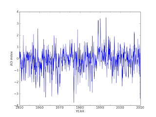
北極振動

最近、寒いのは北極振動が負になっているのが関係しているらしい。
北極振動　wikipedia
http://ja.wikipedia.org/wiki/%E5%8C%97%E6%A5%B5%E6%8C%AF%E5%8B%95
http://en.wikipedia.org/wiki/Arctic_oscillation

AOのデータは以下から入手できる。
http://www.cpc.ncep.noaa.gov/products/precip/CWlink/daily_ao_index/ao.shtml

プロットしてみる

以下プログラム(python)。scikits.timeseriesを使っている。

readAO.py

def readAO():
    "import monthly AO data"

    import numpy as np
    import scikits.timeseries as ts

# data is downloaded from http://www.cpc.ncep.noaa.gov/products/precip/CWlink/daily_ao_index/monthly.ao.index.b50.current.ascii
    f=open("monthly.ao.index.b50.current.ascii",'r')
    data=np.loadtxt(f)
    f.close()

    AOindex=data[:,2]
    year=data[:,0]
    month=data[:,1]

# make time series
    tbeginmonth=str(int(year[0]))+"-"+str(int(month[0]))
    dbeginmonth=ts.Date('M', tbeginmonth)
    AOindex_series=ts.time_series(AOindex,start_date=dbeginmonth,freq='M',mask=(AOindex<-99.))

    return AOindex_series
##################################

if __name__ == '__main__':
    import matplotlib.pyplot as plt
    import scikits.timeseries as ts
    import scikits.timeseries.lib.plotlib as tpl
    from datetime import datetime

    AOindex_series=readAO()

    fig = tpl.tsfigure()
    fsp = fig.add_tsplot(111)
    fsp.tsplot(AOindex_series, '-')

    istart=fsp.get_xlim()[0]
    iend=ts.Date('M','2010-1').value
    fsp.set_xlim(istart,iend)
    plt.xlabel("YEAR")
    plt.ylabel("AO index")
    plt.savefig("AOindex.png")
    plt.show()